Accuracy
Binary classification
$$ y = \left[\begin{array}{l}{0} \\ {1} \\ {0} \\ {1}\end{array}\right], \hat{y} = \left[\begin{array}{l}\textcolor{#228B22}{0} \\ \textcolor{#228B22}{1} \\ \textcolor{#228B22}{0} \\ {0}\end{array}\right] $$
$$ \text{accuracy} = \frac{\textcolor{#228B22}{\text{no. of matches}}}{\#total} = \frac{3}{4} $$
Multiclass classification
$$ y = \left[\begin{array}{l}{0} \\ {2} \\ {1} \\ {3}\end{array}\right], \hat{y} = \left[\begin{array}{l}\textcolor{#228B22}{0} \\ {1} \\ {2} \\ \textcolor{#228B22}{3}\end{array}\right] $$
$$ accuracy = \frac{\textcolor{#228B22}{\#same}}{\#total} = \frac{2}{4} $$
Multilabel binary classification
$$ y = \left[\begin{array}{l}{[0,1,1,0]} \\ {[1,1,0,1]}\\ {[1,0,1,0]}\end{array}\right], \hat{y} = \left[\begin{array}{l}{[0,1,1,1]} \\ \textcolor{#228B22}{[1,1,0,1]}\\ {[0,1,0,1]}\end{array}\right] $$
$$ accuracy = \frac{\textcolor{#228B22}{\#\text{exact matches}}}{\text{\#samples}} = \frac{1}{3} $$
Precision
Ability of classifier to label positives correctly
Binary classification
$$ y = \left[\begin{array}{l}\textcolor{#D8D8D8}{0} \\ {1} \\ {1} \\ \textcolor{#D8D8D8}{0} \\ {0}\end{array}\right], \hat{y} = \left[\begin{array}{l}\textcolor{#D8D8D8}{0} \\ \textcolor{#228B22}{1} \\ \textcolor{#228B22}{1} \\ \textcolor{#D8D8D8}{0} \\ \textcolor{#FF0000}{1}\end{array}\right] $$
$$ precision = \frac{\textcolor{#228B22}{tp}}{\textcolor{#228B22}{tp} + \textcolor{#FF0000}{fp}} = \frac{2}{2+1} $$
Multiclass classification
Micro precisionIdentical to accuracy in multiclass setting.
$$ y = \left[\begin{array}{l}{0} \\ {1} \\ {2} \\ {0}\\ {1}\\ {2}\end{array}\right], \hat{y} = \left[\begin{array}{l}\textcolor{#228B22}{0} \\ {2} \\ {1} \\ \textcolor{#228B22}{0}\\ {0}\\ {1}\end{array}\right] $$
$$ precision_\text{micro} = \frac{\textcolor{#228B22}{\#same}}{\#total} = accuracy = \frac{2}{6} $$
Macro precision
$$ y = \left[\begin{array}{l}{0} \\ {2} \\ {2} \\ {0}\\ {1}\\ {2}\end{array}\right], \hat{y} = \left[\begin{array}{l}\textcolor{#3b70c8}{0} \\ \textcolor{#FFA500}{2} \\ \textcolor{#975f8a}{1} \\ \textcolor{#3b70c8}{0}\\ \textcolor{#3b70c8}{0}\\ \textcolor{#975f8a}{1}\end{array}\right] $$
$$ precision_\text{macro} = \frac{1}{|L|} \sum_{l \in L} \frac{|y_l \cap \hat{y}_l|}{|\hat{y}_l|} = \frac{1}{3} (\textcolor{#3b70c8}{\frac{2}{3}}+\textcolor{#975f8a}{\frac{0}{2}}+\textcolor{#FFA500}{\frac{1}{1}}) = \frac{5}{9} $$
Multilabel binary classification
Micro precision
$$ y = \left[\begin{array}{l}{[0,1,1,0]} \\ {[1,1,0,1]}\\ {[1,0,1,0]}\end{array}\right], \hat{y} = \left[\begin{array}{l}{[0,\textcolor{#228B22}{1},\textcolor{#228B22}{1},\textcolor{#FF0000}{1}]} \\ [\textcolor{#228B22}{1},\textcolor{#228B22}{1},0,\textcolor{#228B22}{1}]\\ {[0,\textcolor{#FF0000}{1},0,\textcolor{#FF0000}{1}]}\end{array}\right] $$
$$ precision_\text{micro} = \frac{\textcolor{#228B22}{\text{no. of 1's in }\hat{y} \text{ that match those in } y}}{\text{no. of 1's in } \hat{y}} = \frac{5}{8} $$
Macro precision
$$ y = \left[\begin{array}{l}{[0,1,1,0]} \\ {[1,1,0,1]}\\ {[1,0,1,0]}\end{array}\right], \hat{y} = \left[\begin{array}{l}{[0,1,1,1]} \\ \textcolor{#228B22}{[1,1,0,1]}\\ {[0,1,0,1]}\end{array}\right] $$
Note: There are 4 labels in each sample. Calculate the precision for one label at a time, then take the average of all the 4 labels.
$$ precision_\text{macro} = \frac{1}{|L|} \sum_{l \in L} \frac{|y_l \cap \hat{y}_l|}{|\hat{y}_l|} = \frac{1}{4}(\frac{1}{1}+\frac{2}{3}+\frac{1}{1}+\frac{1}{3}) = \frac{3}{4} $$
Recall
Ability of classifier to recover the positives
Binary classification
$$ y = \left[\begin{array}{l}\textcolor{#D8D8D8}{0} \\ {1} \\ \textcolor{#D8D8D8}{0} \\ {1} \\ {1}\end{array}\right], \hat{y} = \left[\begin{array}{l}\textcolor{#D8D8D8}{0} \\ \textcolor{#228B22}{1} \\ \textcolor{#D8D8D8}{0} \\ \textcolor{#FF0000}{0} \\ \textcolor{#FF0000}{0}\end{array}\right] $$
$$ recall = \frac{\textcolor{#228B22}{tp}}{\textcolor{#228B22}{tp} + \textcolor{#FF0000}{fn}} = \frac{1}{1+2} $$
Multiclass classification
Micro recallIdentical to accuracy in multiclass setting.
$$ y = \left[\begin{array}{l}{0} \\ {1} \\ {2} \\ {0}\\ {1}\\ {2}\end{array}\right], \hat{y} = \left[\begin{array}{l}\textcolor{#228B22}{0} \\ {2} \\ {1} \\ \textcolor{#228B22}{0}\\ {0}\\ {1}\end{array}\right] $$
$$ precision_\text{micro} = \frac{\textcolor{#228B22}{\#same}}{\#total} = accuracy = \frac{2}{6} $$
Macro recall
$$ y \left[\begin{array}{l}\textcolor{#3b70c8}{0} \\ \textcolor{#FFA500}{2} \\ \textcolor{#FFA500}{2} \\ \textcolor{#3b70c8}{0}\\ \textcolor{#975f8a}{1}\\ \textcolor{#FFA500}{2}\end{array}\right] \left[\begin{array}{l}{0} \\ {2} \\ {1} \\ {0}\\ {0}\\ {1}\end{array}\right] \hat{y} $$
$$ precision_\text{macro} = \frac{1}{|L|} \sum_{l \in L} \frac{|y_l \cap \hat{y}_l|}{|y_l|} = \frac{1}{3} (\textcolor{#3b70c8}{\frac{2}{2}}+\textcolor{#975f8a}{\frac{0}{1}}+\textcolor{#FFA500}{\frac{1}{3}}) = \frac{4}{9} $$
Multilabel binary classification
Micro recall
$$ y = \left[\begin{array}{l}{[0,\textcolor{#228B22}{1},\textcolor{#228B22}{1},0]} \\ [\textcolor{#228B22}{1},\textcolor{#228B22}{1},0,\textcolor{#228B22}{1}]\\ {[\textcolor{#FF0000}{1},0,\textcolor{#FF0000}{1},0]}\end{array}\right] , \left[\begin{array}{l}{[0,1,1,0]} \\ {[1,1,0,1]}\\ {[0,1,0,1]}\end{array}\right] $$
$$ recall_\text{micro} = \frac{\textcolor{#228B22}{\text{no. of 1's in }y \text{ that match those in } \hat{y}}}{\text{no. of 1's in } y} = \frac{5}{7} $$
Macro recall
$$ y = \left[\begin{array}{l}{[0,1,1,0]} \\ {[1,1,0,1]}\\ {[1,0,1,0]}\end{array}\right], \hat{y} = \left[\begin{array}{l}{[0,1,1,1]} \\ \textcolor{#228B22}{[1,1,0,1]}\\ {[0,1,0,1]}\end{array}\right] $$
Note: There are 4 labels in each sample. Calculate the recall for one label at a time, then take the average of all the 4 labels.
$$ precision_\text{macro} = \frac{1}{|L|} \sum_{l \in L} \frac{|y_l \cap \hat{y}_l|}{|y_l|} = \frac{1}{4}(\frac{1}{2}+\frac{2}{2}+\frac{1}{2}+\frac{1}{1}) = \frac{3}{4} $$
F1
Binary classification
$$ f1 = 2 \cdot \frac{precision \times recall}{ precision + recall} $$
Multiclass classification
Micro F1Identical to accuracy in multiclass setting.
$$ f1_{\text{micro}} = 2 \cdot \frac{precision_{\text{micro}} \times recall_{\text{micro}}}{ precision_{\text{micro}} + recall_{\text{micro}}} = accuracy$$
Macro F1
$$ f1_{\text{macro}} = 2 \cdot \frac{precision_{\text{macro}} \times recall_{\text{macro}}}{ precision_{\text{macro}} + recall_{\text{macro}}} $$
Multilabel binary classification
Micro F1
$$ f1_{\text{micro}} = 2 \cdot \frac{precision_{\text{micro}} \times recall_{\text{micro}}}{ precision_{\text{micro}} + recall_{\text{micro}}}$$
Macro F1
$$ f1_{\text{macro}} = 2 \cdot \frac{precision_{\text{macro}} \times recall_{\text{macro}}}{ precision_{\text{macro}} + recall_{\text{macro}}} $$
AUC / AUROC (Area Under Curve / Area Under ROC)Your predicted values must be scores.
ROC is plotted on a graph of TPR over FPR, and the area below this graph is called area under curve (AUC). AUC represents the probability that a random positive example is positioned to the right of a random negative example. See here.
Suppose
$$ y = \left[\begin{array}{l}{0} \\ {0} \\ {1}\end{array}\right], \hat{y} = \left[\begin{array}{l}{0.8} \\ {0.3} \\ {0.6}\end{array}\right] $$
Use 4 different thresholds, above any of which will be considered positive, below of which negative. Here we chose [1.8, 0.8, 0.6, and 0.3].
Threshold = 1.8
$$ y = \left[\begin{array}{l}{0} \\ {0} \\ {1}\end{array}\right], \hat{y} = \left[\begin{array}{l}\textcolor{#76BED0}{0} \\ \textcolor{#76BED0}{0} \\ \textcolor{#F4A261}{0} \end{array}\right] $$
$$ fpr = \frac{\textcolor{#FF0000}{fp}}{\textcolor{#FF0000}{fp} + \textcolor{#76BED0}{tn}} = \frac{0}{0+2} = 0 $$
$$ tpr = \frac{\textcolor{#228B22}{tp}}{\textcolor{#228B22}{tp} + \textcolor{#F4A261}{fn}} = \frac{0}{0+1} = 0 $$
Threshold = 0.8
$$ y = \left[\begin{array}{l}{0} \\ {0} \\ {1}\end{array}\right], \hat{y} = \left[\begin{array}{l}\textcolor{#FF0000}{1} \\ \textcolor{#76BED0}{0} \\ \textcolor{#F4A261}{0}\end{array}\right] $$
$$ fpr = \frac{\textcolor{#FF0000}{fp}}{\textcolor{#FF0000}{fp} + \textcolor{#76BED0}{tn}} = \frac{1}{1+1} = \frac{1}{2} $$
$$ tpr = \frac{\textcolor{#228B22}{tp}}{\textcolor{#228B22}{tp} + \textcolor{#F4A261}{fn}} = \frac{0}{0+1} = 0 $$
Threshold = 0.6
$$ y = \left[\begin{array}{l}{0} \\ {0} \\ {1}\end{array}\right], \hat{y} = \left[\begin{array}{l}\textcolor{#FF0000}{1} \\ \textcolor{#76BED0}{0} \\ \textcolor{#228B22}{1}\end{array}\right] $$
$$ fpr = \frac{\textcolor{#FF0000}{fp}}{\textcolor{#FF0000}{fp} + \textcolor{#76BED0}{tn}} = \frac{1}{1+1} = \frac{1}{2} $$
$$ tpr = \frac{\textcolor{#228B22}{tp}}{\textcolor{#228B22}{tp} + \textcolor{#F4A261}{fn}} = \frac{1}{1+0} = 1 $$
Threshold = 0.3
$$ y = \left[\begin{array}{l}{0} \\ {0} \\ {1}\end{array}\right], \hat{y} = \left[\begin{array}{l}\textcolor{#FF0000}{1} \\ \textcolor{#FF0000}{1} \\ \textcolor{#228B22}{1}\end{array}\right] $$
$$ fpr = \frac{\textcolor{#FF0000}{fp}}{\textcolor{#FF0000}{fp} + \textcolor{#76BED0}{tn}} = \frac{2}{2+0} = 1 $$
$$ tpr = \frac{\textcolor{#228B22}{tp}}{\textcolor{#228B22}{tp} + \textcolor{#F4A261}{fn}} = \frac{1}{1+0} = 1 $$
And so you have a list of fpr's and tpr's.
For multilabel binary classification
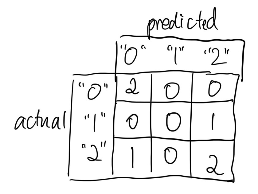
Confusion matrix